
What is a Neural Network?
Artificial Neural Networks (ANNs) are information processing systems that are inspired by the biological neural networks like a brain. They are a chain of algorithms which attempt to identify relationships between data sets.
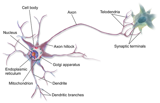
In its simplest form, a biological brain is a huge collection of neurons. Each neuron takes electrical and chemical signals as inputs through its many dendrites and transmits the output signals through its axon (in a more specialized context, there are exceptions to this behavior like with multipolar neurons). Axons make contact with other neurons at specialized junctions called synapses where they pass on their output signals to other neurons to repeat the same process over and over millions and millions of times.
Taking inspiration from the brain, an artificial neural network is a collection of connected units, also called neurons. The connection between the neurons can carry signals between them. Each connection carries a real number value which determines the weight/strength of the signal.
ANNs are universal function approximators who at there very essence attempt to approximate a function/relation between the input data and the output data.
Neurons
Neurons are the basic building blocks of ANNs. An artificial neuron receives vectorized input and operates on them to produce vectorized output. This is similar to dendrites in a biological neuron receiving input signals and sending out an output signal through its axon.
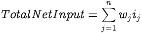
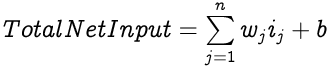
Each input to an artificial neuron is individually weighted to determine the strength of each input. A weighted summation of all the inputs with their weights forms the total net input to a neuron. For a neuron with n inputs i and the same number of corresponding weights w, the Total Net Input would be:
Consider the following diagram of an artificial neuron.

In the above artificial neuron, i1 and i2 are the inputs to the neuron where each input has weights w1 and w2 respectively. Hence, the Total Net Input for the neuron would be:

The neuron then computes the output using an activation function on the Total Net Input. The result of the activation function is the output of the neuron.

The output of a neuron is forwarded to the next neuron in line as input. In an ANN, the results from one layer of neurons are progressively forwarded to the neurons in the next layer until they exit from the output layer as the output of the network.
Activation Functions
The Total Net Input to a neuron could be anywhere between +Infinity to -Infinity. To decide whether the neuron should fire/activate (i.e. generate an output) researchers introduced activation functions inside neurons. Activation functions provide complex non-linear functional mapping between the net inputs and output of a neuron.
Without the activation functions, the output of a neuron will just be a linear function of the input parameters. An ANN without an activation function is a Linear Regression Model i.e. polynomial function of degree one. Though, it would be much easier to train such an ANN, they would be limited in their complexity and have less capability to learn complex functional mappings from complex non-linear data sets like images, audio, video etc.
Similarly, having linear activation functions would also give us a linear neural network of input parameters regardless of how many hidden layers we add in the network.
Unlike linear functions, non-linear functions are polynomials functions of a degree more than one and their plottings on a map are curved. For an ANN to be able to create non-linear arbitrary and complex mappings between the input and output, we need non-linear activation functions.
Another important requirement for an activation function is that it should be differentiable so that we can calculate the error gradient of the network with respect to its weights. This gradient is needed to perform back propagation optimization strategy as we will soon see.
Some of the most popular activation functions are:
Every activation function has its own characteristics, for example Sigmoid suffers from the vanishing gradient problem and the zero-centered problem. Tanh solves the zero-centered problem but suffers from the vanishing gradient problem. ReLU helps in solving the vanishing gradient problem but it too suffers from the zero-centered problem.
Recently, ReLU has become the popular choice as activation function for hidden layer neurons.
The choice of activation function inside a neuron heavily influences the learning techniques employed on the network and vice versa.
Though Sigmoid has fallen out of favor with neural network designers nowadays, we would be using it in the current implementation.
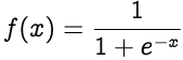
The sigmoid function non-linearly squashes or normalizes the input to produce an output in a range of 0 to 1.
Topology Of an Artificial Neural Network
The neurons in an ANN are arranged in two layers vis hidden layer and output layer. In addition to these two layers, there is also a third layer called the input layer which doesn't has any neurons but instead just acts as a vector or matrix for the input data.
One of the simplest form of neural networks is a single hidden layer feed forward neural network.
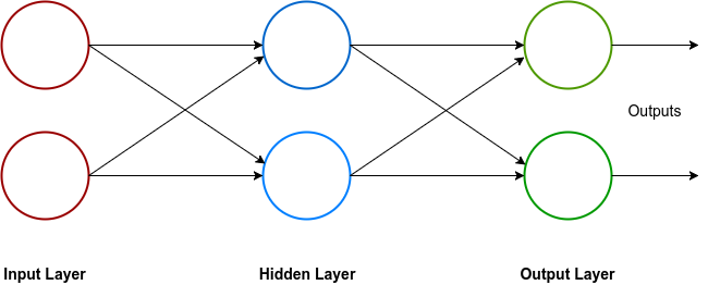
All the directed connections in a neural network are meant to carry output from one neuron to the next neuron as input. All these connections are weighted to determine the strength of the data they are carrying.
Multi Layer Perceptrons (MLP)
MLPs are one of the most popular topologies of neural networks being used today. MLPs have only one input and output layer but can have more than one hidden layers. Each layer in MLPs can have numerous nodes.
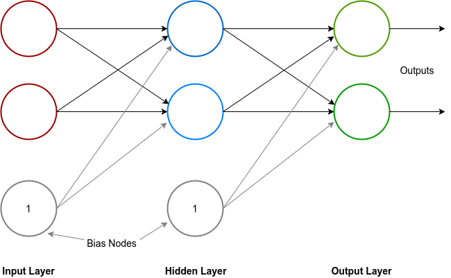
In addition to the neurons, each layer except the output layer also has a bias node. The bias node in a layer also has weighted connections with neurons of the next layer but its input value is always 1, hence the weight of the connection is the effective input from the bias to the neuron. The Total Net Input to a neuron with n inputs and a bias is:
Where w and i are the weight and input respectively while b is the weight from the bias node to the neuron.
All inputs from the input layer along with the bias are forwarded to each neuron in the hidden layer where each neuron performs a weighted summation of the input and sends the activation results as output to the next layer. The process repeats until the data final exits form the network through the output layer. This process is called the feed forward process.
Why do we need bias nodes?
As mentioned before, neural networks are universal function approximators and they assist us in finding a function/relationship between the input and the output data sets. In a neural network without bias nodes, the output is the result of a direct function of the inputs of the network without any constant to adjust the shift in the output.
To understand better, consider the geometric equation of a line passing through the origin on a 2D cartesian plane:

Here, m is the slope of the line and x & y hold the coordinates of the points on the line.
For a line not passing through the origin, a new constant c (also called the y-intercept) is introduced in the equation to quantify the shift in the line away from the origin. The y-intercept is not related to any of the coordinates.

For the line passing through the origin, we can train a neural network without bias nodes to estimate the y coordinate of a point if the x coordinate is given. After training, the weights in the neural network will get adjusted to emulate the value of the slope m. But such a network will not be able to learn, with reasonable accuracy, from a coordinates set of a line not passing through the origin because there are no weights unrelated to the input to emulate the behavior of the constant c. Each weight in the network is directly or indirectly related to the input of the network.
A neural network with bias nodes however can learn to predict the coordinates of a line not passing through the origin. With training, the weights of the bias nodes will also get adjusted to emulate the behavior of the y-intercept c.
Back Propagation Algorithm
Back propagation algorithm is a supervised learning algorithm which uses gradient descent to train multi-layer feed forward neural networks.
The back propagation algorithm involves calculating the gradient of the error in the network's output against each of the network's weights and adjusting the weights to reduce the error. In simpler words, it calculates how much effect each weight in the network has on the network's error and adjusts every weight to reduce the error.
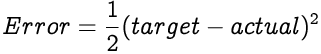
The error value indicates how much the network's output (actual) is off the mark from the expected output (target). We use the Mean Squared Error function to calculate the error.
The error value of a single output neuron is a function of its actual value and the target value.
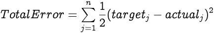
The total error of the network is a sum of all error values from all output neurons. For a network with n neurons in the output layer, the Total Error is:
To understand the back propagation algorithm, consider a single output neuron with only one input connection. The input data would follow the following flow to give us the total network error.

To calculate the gradient of the Total Error against a weight, we calculate the partial differential of the Total Error with respect to the weight.
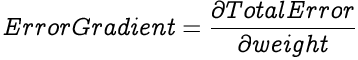
We employ the chain rule to simplify the above equation by splitting it into smaller equations.

Let's look into solving each of the individual differentials to get the initial desired differential.
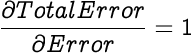
The Total Error of a network is the sum of errors in all its output neurons. Since we are calculating the partial differential with respect to only one neuron's error, errors from other neurons are treated as constants since they are not a function of the selected neuron's error, hence they don't effect the partial differential. So essentially we are calculating the partial differential of an entity against itself, hence the partial differential of Total Error with respect to one neuron's error is 1.
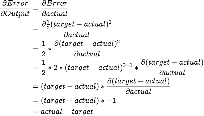
As mentioned earlier, we use the Mean Squared Error function to calculate the error in an output neuron's actual output.
Since, actual is the output of the neuron, the derivative of the error with respect to the Output would be:
As we are using the Sigmoid activation function to calculate output from the Total Net Input, which is a function of only one variable, we calculate the derivative instead of partial derivative of a neuron's output with respect to its input using this formula.

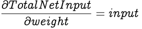
As we already know, the Total Net Input of a neuron is a weighted summation of all its inputs and the bias. The derivative of the Total Net Input with respect to one of its weights is the corresponding input factor of that particular weight since all other weighted sums and bias will be treated as constants.
After solving for each of the individual differentials, we can now calculate the partial differential of the Total Error with respect to a weight. Once we have that, we adjust our weight in proportion to the learning rate.

The learning rate determines how drastically do the weights in a network get adjusted based on the error differential. In other words, how quickly or slowly will the neural network adapt to reduce its errors. The learning rate's value spans between 0 and 1. There are caveats for using both high and low learning rates.
If a neural network's learning rate is too high then it will quickly adjust it weights for any errors in the output. As a consequence, the latest data set in the training data set will have a much higher bearing on the network's output than the earlier data sets. In simpler words, the network will readily learn from the latest data but will keep forgetting lessons from the older data.
On the other hand, having a very low learning rate is also fraught with consequences. The network will have a higher inertia against learning i.e. it will be very slow to responding to any errors in the output. As a result, it will either only learn in the beginning and become prejudiced against the later training data sets or it will not learn at all and will remain stuck with the initial weights it was initialized with.
We just saw how back propagation of errors is used in MLP neural networks to adjust weights for the output layer to train the network. We use a similar process to adjust weights in the hidden layers of the network which we would see next with a real neural network's implementation since it will be easier to explain it with an example where we have actual numbers to play with.
Neural Network Implementation
Let's build a neural network and train it to approximate the function for a XOR gate. The following are the I/O sets for a XOR gate:
| A | B | A XOR B |
|---|---|---|
| 0 | 0 | 0 |
| 0 | 1 | 1 |
| 1 | 0 | 1 |
| 1 | 1 | 0 |
As we can see a XOR gate accepts two inputs and returns a single output. Hence we need a neural network with two input nodes and one output neuron. We will also opt to use two neurons in the hidden layer of our neural network. Determining the number of neurons needed in the hidden layer depends on a wide variety of variables and there are a number of hidden layer configuration designs to choose from.
The general consensus is that, if the number of inputs is greater than the outputs, the number of neurons in the hidden layer should be between the number of nodes in the input and the output layer but never greater than the number of input nodes. The last bit exists so that the network can generalize better instead of overfitting/memorizing the training data.
Since we know the expected output for our inputs, this will be called supervised learning. Also, since we will be predicting the output value for the input set, we are creating a regression neural network model.
Apart from neurons we will also add one bias node in the input and the hidden layer.
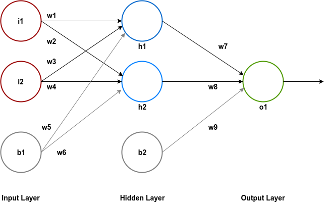
Notice that we have labeled all the nodes and the weights in the network for easy of explanation.
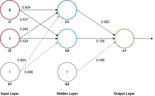
The next step is to initialize all the connections between the neurons of different layers with weights. Initially these weights are just random decimal point numbers between 0 and 1.
Let us start training our network with the second row in the above table. The input nodes will have the values 0 & 1.
Now that we have initialized our network let us see what output it spews out for the selected input.
Feed Forward
Hidden Layer
We need to calculate the Total Net Input to each hidden layer neuron, squash it using the activation function and then repeat the same process for the output layer.
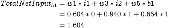
First let's calculate the Total Net Input to the first hidden layer neuron, h1.
As described earlier, the Total Net Input to a neuron is a weighted summation of all of its inputs and its bias. Hence, the Total Net Input to h1 is:
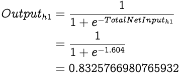
Now that we have the Total Net Input to h1 we can calculate the Output from h1 using the sigmoid function:
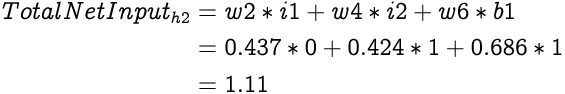
Similarly, the Total Net Input to the second hidden layer neuron, h2 will be:
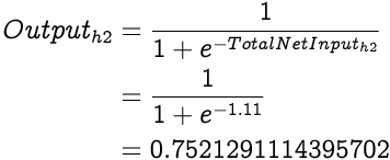
And the Output from h2 is:
As we know, in a feed forward neural network, output from one layer is input to the next layer. So now let's input our hidden layer outputs in the output layer.
Output Layer
We begin by calculating the Total Net Input to the output layer's neuron, o1.

The Output from o1 would be:
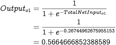
0.5664666852388589 is the output from the neural network for the given inputs 0 and 1 while the expected output is 1. As expected from the first run of a neural network, the actual output is quite the way off from the target output since we are operating with random weights.
Back propagation
Now we will employ back propagation strategy to adjust weights of the network to get closer to the required output.
We will be using a relatively higher learning rate of 0.8 so that we can observe definite updates in weights after learning from just one row of the XOR gate's I/O table. Generally a starting learning rate of 0.5 is used in most applications. I say starting rate because many back propagation techniques nowadays also update the learning rate as the training progresses. Another interesting concept is to use a variable learning rate based on the actual output's deviation from the target output instead of a fixed learning rate. For the sake of simplicity we will only be using a fixed learning rate in our implementation.
As we know, the Total Error from a neural network is simply a sum of errors from all the output neurons. Since we have only one output neuron in our network, the Total Error is simply the error from output neuron o1.

Let us begin updating weights to the output layer.
Output Layer
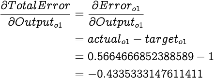
First we calculate the partial differential of Total Error from the network with respect to the Output of output layers only neuron o1. Hence, the partial differential of Total Error with respect to Output of o1 is:
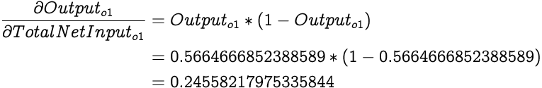
Next we need a derivative of Output of o1 with respect to the Total Net Input to o1. From what we earlier discussed:
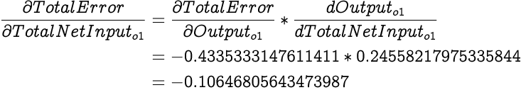
Now from our understanding of chain rule:
We now have the partial differential of Total Error with respect to the Total Net Input to the output neuron. To adjust the weights from the hidden layer to the output layer we need to find partial differential of Total Error with respect to each of those individual weights and update them.
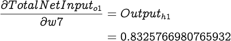
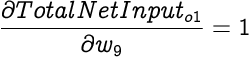
Next we calculate the partial differential of Total Net Input with respect to each of the weights (i.e. w7, w8 and w9). As we know from earlier explanations, partial differential of Total Net Input with respect to the weight is simply the input associated with that weight when calculating the Total Net Input. Therefore,
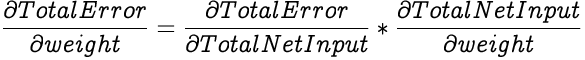
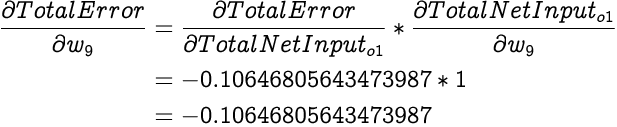
And according to the chain rule, we can express partial differential of Total Error with respect to weight as:
Building on the above equation,
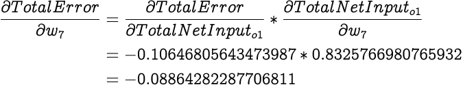
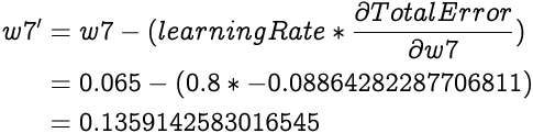
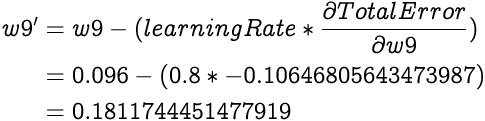
Now that we know how much the Total Error of the network is affected by the weight w7, we can use this to set a new value for w7:
Similarly, partial differential of Total Error with respect to w8 is:
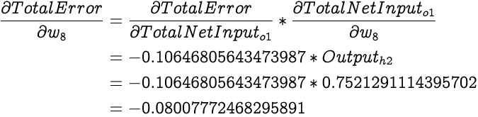
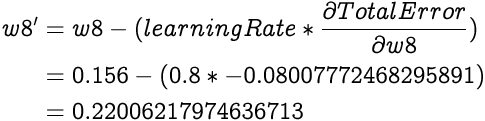
We can now update w8 as:
There is also a third weight from the hidden layer to the output layer, w8. But unlike the above weights, this is not on a connection from a hidden layer neuron but instead from a bias node. Fortunately, updating this weight is also very much like updating the previous weights.
As we discussed earlier, the partial differential of Total Net Input with respect to a weight is simply the corresponding input associated with that weight. Since, the output from a bias node is always 1, the associated input in this case is also 1. Hence,
Now we can calculate the partial differential of Total Error with respect to this weight, which as per the chain rule can be expressed as:
Hence we can adjust the weight w8 on the connection from the bias node as:
Updating the weights from the hidden layer to the output layer with the new weights should bring the output closer to the target output thereby reducing the network's error.
To further improve the network's output we also update the weights from the input layer to the hidden layer.
Hidden Layer
Like with the output layer, to update weights we calculate how much the change in the weights affects the Total Error of the network. i.e. we calculate the partial differential of error with respect to each of the hidden layer weights.
First we calculate the partial differential of Total Error with respect to a hidden neuron's output which can be expressed with the following equation for an output layer with n neurons.

Note that since the output from a hidden neuron is fed into each of the output layer neuron and the Total Error is a summation of errors from each of the output neuron, the partial differential of Total Error with respect to the output of a hidden neuron is a summation of chain rule calculations via Total Net Input of each of the output layer neuron.
Now since our network has only a single output neuron, we can calculate the partial differential of Total Error with respect to the output of h1 as:

We have already calculated partial differential of Total Error with respect to the Total Net Input to o1 in the previous section. The output from h1 is one of the inputs to o1, and from our earlier discussions we know that partial differential of Total Net Input with respect to an input is the weight corresponding to the input while calculating the input. Therefore,
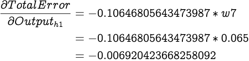
Notice that we used the old value of w7 not the new one because we are still calculating gradient for the error generated while the old weight was being used.
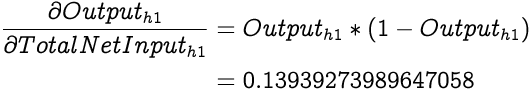
Moving on in our chain, we next calculate the derivative of output from h1 with respect to the Total Net Input to h1. The output, as we already know, is generated by squashing the input with the sigmoid function. Hence, the derivative is a derivative of the sigmoid function which as we have discussed earlier is:
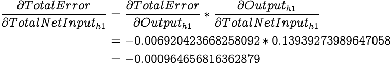
Now that we have the necessary elements to calculate the partial differential of Total Error with respect to the Total Net Input to h1, we calculate it by first simplifying it using the chain rule:
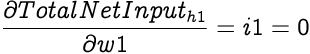
The Total Net Input to h1 is a function of inputs from i1, i2 and b1 with w1, w3 and w5 as the corresponding weights respectively. We will now find new values for weights w1 and w3 from input nodes and w5 from the bias node.
As we know, the partial differential of Total Net Input with respect to a weight is simply the input value corresponding to the weight. Therefore,
Again applying the chain rule,
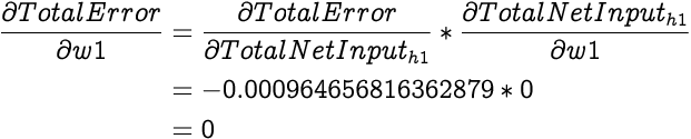
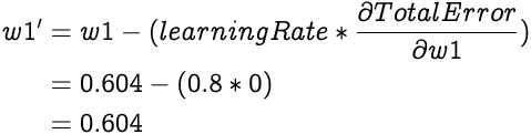
Now that we know how much the weight w1 affects the Total Error, we can adjust it to minimize the Total Error. Since the affect of w1 on the Total Error is zero the new weight should remain unchanged. This can be validated by applying the weight update equation.
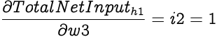
We can use a similar approach to calculate how much the partial differential of Total Net Input to h1 with respect to w3,
Hence,

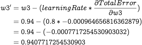
Now similar to w1 we can calculate new weight for w3 as:
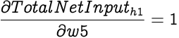
As with weights from the input nodes, we also need to update weight w5 from the bias node b1. First we find out how much the weight w5 affects the Total Net Input to h1. Since the corresponding input for the w5 in equation for calculating the Total Net Input is 1,
Hence,
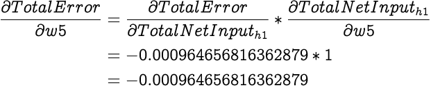
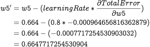
Calculating the new value for weight w5:
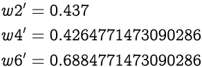
Using the above techniques to calculate new values for weights from input layer to h2, we get the following values:
Conclusion
If we again employ the feed forward technique to the neural network for the same input but with the new weights, we get 0.6130333654357785 as output. Which is slightly closer to the target output of 1 compared to the earlier output 0.5664666852388589. This is essentially how a neural network training works, over several iterations with randomly selected input data the network gradually updates its weight to reduce its total error. The choice of learning rate, number of hidden neurons, activation functions etc, dictate the speed and accuracy of the network's training life cycle.
Example
You can experiment with a basic GoLang based back propagation implementation I have on GitHub at: surenderthakran/back-propagation-demo where I train a neural network to learn the AND gate.
You can also checkout my attempt at writing a neural network library at surenderthakran/gomind which I hope will take a respectable shape in the coming weeks.